Getting X8 photon count data to agree with numerical prediction for beamsplitter phase sweep

[adidasty]

I am using the X8 to compare the Fock probabilities \vert {}_{0145}\langle 0,1,0,1\vert U_{\text{BS}}({\pi\over 4},\varphi)_{01}U_{\text{BS}}({\pi\over 4},\varphi)_{45}\vert \text{TMSS}_{r=1}\rangle_{04}\vert \text{TMSS}_{r=1}\rangle_{15}\vert^{2} and \vert {}_{0145}\langle 0,1,0,1\vert \vert \text{TMSS}_{r=1}\rangle_{04}\vert \text{TMSS}_{r=1}\rangle_{15}\vert^{2} on the interval \varphi \in [-{\pi\over 2},{\pi\over 2}].

To compare these probabilities, I get the respective empirical estimates Q(\varphi) and P and calculate \vert 1-{Q(\varphi)\over P}\vert. The analytical version of this function and the numerical simulation (with MeasureFock and TensorFlow backend and cutoff=10) are shown below. (Well, I can only put one image in a post, so just believe me that the photon counting simulation matches the analytical result {1\over 2}-{1\over 2}\cos 2\varphi).

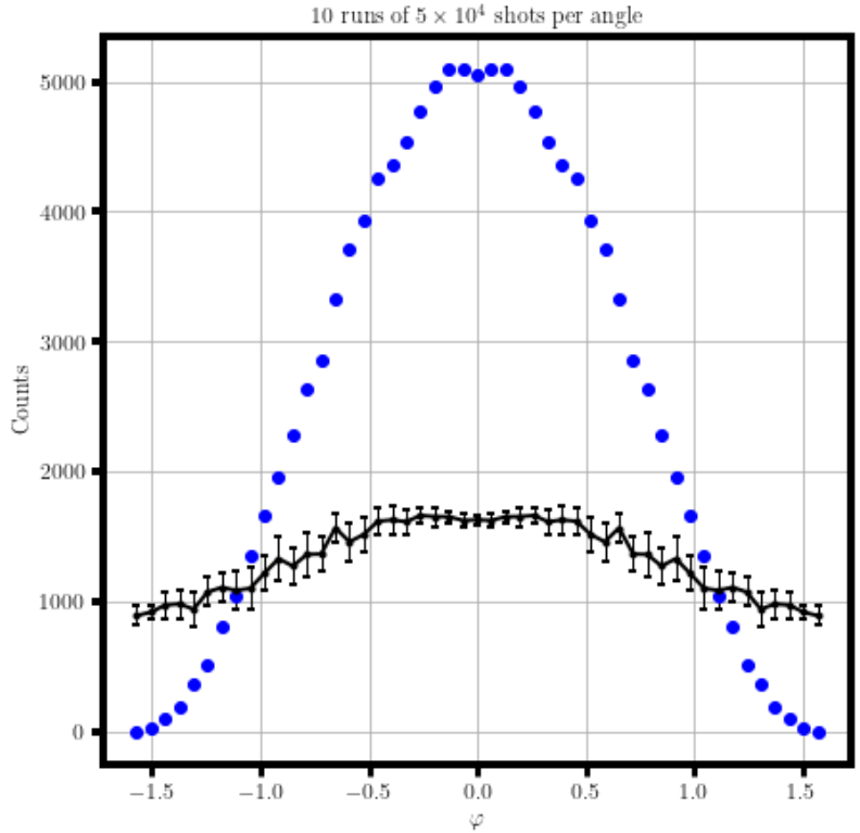
On the X8, I’m unable to get the expected value of this function correct (especially near \pm {\pi\over 2} and 0), see below (I’ve just reflected the [-{\pi\over 2},0] data about 0).

In both cases, I estimate the probability of \vert 0,1,0,1\rangle_{0145} by summing all photon counts that agree with 0,1,0,1 on modes 0145.

Code for Q(\varphi):

sf.ops.S2gate(1.0) | (q[0], q[4])
sf.ops.S2gate(1.0) | (q[1], q[5])
sf.ops.BSgate(np.pi/4, phi) | (q[0], q[1])
sf.ops.BSgate(np.pi/4, phi) | (q[4], q[5])
sf.ops.MeasureFock() | q
eng = sf.RemoteEngine(“X8”)
return eng.run(prog, shots=n_samples,disable_port_permutation=True)

Code for P:

sf.ops.S2gate(1.0) | (q[0], q[4])
sf.ops.S2gate(1.0) | (q[1], q[5])
sf.ops.MeasureFock() | q
eng = sf.RemoteEngine(“X8”)
return eng.run(prog, shots=n_samples,disable_port_permutation=True)

The fact that near \pm {\pi\over 2}, the function is about half what it should be makes me think I’ve coded something wrong. Is there a way that I could get the X8 calculation to match the analytical result more closely?

[CatalinaAlbornoz]

Hi @adidasty, welcome to the forum and thank you for your question!

We’re looking into it and will be back soon with an answer.

[Tom_Bromley]

Hi @adidasty!

Thanks for your detailed post! My initial reaction would be that both Q(\varphi) and P are being calculated experimentally and taking the ratio Q(\varphi) / P is causing the error to shoot up. Have you tried plotting Q^{\rm experiment}(\varphi) against Q^{\rm simulator}(\varphi) as well as finding P^{\rm experiment} to get an idea of the individual errors?

[adidasty]

Hi Catalina and Tom!

“the ratio…is causing the error to shoot up”

Could be-- and Q and P are coming from the probability of a single Fock state, so there’s no cumulation like in Fig. 3 of Arrazola, et al. “Quantum circuits with many photons…”. If the squeezing were increased beyond r\approx 1.0, it would require many more shots to get a good estimate of Q and P and I would have expected the large error in the quotient.

“Have you tried plotting Q^{\rm experiment}(\varphi) against Q^{\rm simulator}(\varphi) as well as finding P^{\rm experiment} to get an idea of the individual errors?”

Yes, the photon count that gives the Q^{\rm simulator}(\varphi) and Q^{\rm experiment}(\varphi) is below (the simulation is exact if I just increase the cutoff and shots, which is time consuming, so I’m just putting one run data for the blue dots; still 50,000 shots per angle though).

With the approximate value r=1.0, the probability of \vert 0,1,0,1\rangle at \varphi=0 is {\tanh(1)^{2}\over \cosh(1)^{4}}\approx 0.1, so the simulation looks good. The total count of 0,1,0,1 from modes 0145 of the X8 (or from my postprocessing of the raw count data!) is different.

[adidasty]

Speaking of that, I better show the lines I’m using to get the total 0,1,0,1 count for a given \varphi on modes 0145 of the X8 (cv_job is the StrawberryFields code for Q(\varphi) that I posted before):

I apologize in advance if this code for the total 0,1,0,1 count is the issue.

[CatalinaAlbornoz]

Hi @adidasty!
This doesn’t seem to be a software issue. I’ll check with the hardware team to see if we can figure out why this is happening! I hope to have an answer soon.

[CatalinaAlbornoz]

Hi @adidasty! It seems that there are two problems which may be causing this difference.

1 - In your simulation you should account for some loss which is inherent to the experimental result. You can try repeating your simulation with 8dB of loss on all modes and see if the agreement is closer.

2 - On the other hand, there may be a compiler issue happening here. Since the code is not identical (even though the circuits are identical) the compiler is actually programming the QPU differently in the two cases - which can have large effects due to imperfections. You can print out prog.compile(device=eng.device_spec).print(), which gives you the compiled program, and check whether or not they are the same.

We’re trying to find a template that can help you ensure all the phases in the unitary are set to what you think they are set to. In the meantime you can try points 1 and 2 and let me know how it goes!

[CatalinaAlbornoz]

Hi @adidasty!
This is the template, which is basically a pattern for a quantum program

def run_job(id,phases,shots):
    prog = sf.Program(8, name="template")

    with prog.context as q:
        ops.S2gate(1.0) | (q[0], q[4])
        ops.S2gate(1.0) | (q[1], q[5])
        ops.S2gate(1.0) | (q[2], q[6])
        ops.S2gate(1.0) | (q[3], q[7])
        
        ops.MZgate(phases[0], phases[1]) | (q[0], q[1])    
        ops.MZgate(phases[2], phases[3]) | (q[2], q[3])
        ops.MZgate(phases[4], phases[5]) | (q[1], q[2])
        ops.MZgate(phases[6], phases[7]) | (q[0], q[1])       
        ops.MZgate(phases[8], phases[9]) | (q[2], q[3])
        ops.MZgate(phases[10], phases[11]) | (q[1], q[2])  
        ops.MZgate(phases[0], phases[1]) | (q[4], q[5])
        ops.MZgate(phases[2], phases[3]) | (q[6], q[7])
        ops.MZgate(phases[4], phases[5]) | (q[5], q[6])
        ops.MZgate(phases[6], phases[7]) | (q[4], q[5])
        ops.MZgate(phases[8], phases[9]) | (q[6], q[7])
        ops.MZgate(phases[10], phases[11]) | (q[5], q[6])
      
        ops.MeasureFock() | q
        
    eng = sf.RemoteEngine("X8_01")
    prog.print()
    results = eng.run(prog, shots=shots, disable_port_permutation=True)
    
    return results 

Where phases is an array of phases with the following convention:

Let me know if this helps!

[adidasty]

Hi Catalina,

Thanks for discussing with the hardware team and continuing to seek a satisfactory resolution to the discrepancy.

1- I am sure that I can modify the simulation to better match the output of X8, but I am going to focus effort on matching the output of X8 to the simulation to the maximum extent possible.

2- prog.compile tells me that when I specify a BSgate (e.g., on modes 01), it is getting compiled with MZgate and Rgate. So I’ll use the rectangular decomposition (i.e., the decomposition indicated by your schematic) of the BSgate at each angle \phi. This will give me the twelve phases in your program. Once I do this, I’ll test it and report back.

[CatalinaAlbornoz]

Hi @adidasty great! Let us know how it goes!

As for point 1 the goal is to confirm that the result you’re getting is the result that should be expected. You can later remove the loss but at least you’ll know how much of the discrepancy is a result of this loss.

[adidasty]

Hi Catalina,

When I specify the rectangular decomposition U_{\text{BS}}(\theta,\varphi)=e^{i(\varphi+\pi)a^{\dagger}a}U_{\text{MZ}}(\pi -2\theta,2\pi-\varphi) (up to complex multiple of modulus 1), i.e., when I use the circuit

with prog.context as q:
    sf.ops.S2gate(1.0) | (q[0], q[4])
    sf.ops.S2gate(1.0) | (q[1], q[5])
    sf.ops.MZgate(np.pi/2, (2*np.pi)-phi) | (q[0], q[1])
    sf.ops.MZgate(np.pi/2, (2*np.pi)-phi) | (q[4], q[5])
    sf.ops.Rgate(phi+np.pi) | (q[0])
    sf.ops.Rgate(phi+np.pi) | (q[4])
    sf.ops.MeasureFock() | q

I get a cleaner photon count for all angles (lowest black line), as you expected. The other black line is the same data that I showed previously in which I just used BSgates. Does the cleaner photon count look like the best result I can hope to get with the X8?

The blue dots show the noisy simulation with 5\times 10^4 shots (for each angle) given by

with prog.context as q:
    sf.ops.S2gate(1.0) | (q[0], q[2])
    sf.ops.S2gate(1.0) | (q[1], q[3])
    sf.ops.BSgate(np.pi/4, phi) | (q[0], q[1])
    sf.ops.BSgate(np.pi/4, phi) | (q[2], q[3])
    sf.ops.LossChannel(1 - 0.7) | q[0]
    sf.ops.LossChannel(1 - 0.7) | q[1]
    sf.ops.LossChannel(1 - 0.7) | q[2]
    sf.ops.LossChannel(1 - 0.7) | q[3]
    sf.ops.MeasureFock() | q

using the Gaussian engine. Clearly, the photon counts for this simulation are closer to the X8 results than for the noiseless simulation, although the shape of the curve is still different, so maybe LossChannel should be composed with another noise channel to match the X8 better. Or maybe replacing LossChannel by ThermalLossChannel with certain parameters would do better?

[CatalinaAlbornoz]

Hi @adidasty, it seems that the result you have with the X8 is the best you can expect.

Regarding the simulation it seems that the loss is really closer to 0.9 so if you change this value you will likely get a closer result to the actual one. Also, thermal noise is indeed possible so composing it with the loss channel should give you a more realistic simulation.

Let me know how this goes!

[CatalinaAlbornoz]

Hi @adidasty, the thermal photons account for about 1/10 of the total counts so it would be interesting to include thermal noise in your simulation.

[adidasty]

Hi Catalina,

Black dots are the no noise simulation (TF backend). Blue dots are the simulation I showed before with LossChannel(0.3) (Gaussian backend). Green dots are the simulation with ThermalLossChannel(0.9,1) (Gaussian backend), red dots are with ThermalLossChannel(0.9,1.5) (Gaussian backend), cyan dots are with ThermalLossChannel(0.9,2.0) (Gaussian backend). These latter three simulations have a more realistic transmissivity, I think. All simulations are 50,000 shots per angle. The X8 count data is the black line with error bars-- 10 runs of 50,000 shots per angle. It seems that different \varphi values need different loss channels to get a simulation that agrees with the X8 globally. Is there any expectation that the beamsplitter phase should affect the loss? Another question: the black dots are obtained with TF backend with cutoff 10 and 50,000 shots (these counts are quite close to what I expect analytically); but when I run this with the Gaussian backend and same number of shots (either with cutoff 10 or no cutoff specified), I get photon counts that are consistently about 18% higher in the range \varphi\in (-0.5,0.5), but agree well when \varphi is near \pm \pi/2. Any explanation?

Finally, picking out the simulation ThermalLossChannel(0.9,2.0) as the “best match”, I did the cost function simulation (recall the cost function \vert 1-{Q(\varphi)\over P}\vert).

Black dots are no noise, cyan dots are with ThermalLossChannel(0.9,2.0), black line with errorbar is X8 result. The X8 cost function in black is improved compared to my first post because I have explicitly written the rectangular decomposition of the beamsplitter, as we discussed. But I still wanted to know why I don’t get a value near 0 when \varphi is near 0. Doing some test runs leads to an interesting hypothesis: the reason that the cost function does not get close to 0 at \varphi=0 seems to be that P is too big (i.e., X8 returns an empirical value of P that high relative to the values of Q(\varphi); recall that P is computed with the U_{4} element being the identity). If the P from the X8 is replaced by a value for P calculated from a noisy simulation using

sf.ops.S2gate(1.0) | (q[0], q[2])
sf.ops.S2gate(1.0) | (q[1], q[3])
sf.ops.ThermalLossChannel(1 - 0.1,2.0) | q[0]
sf.ops.ThermalLossChannel(1 - 0.1,2.0) | q[1]
sf.ops.ThermalLossChannel(1 - 0.1,2.0) | q[2]
sf.ops.ThermalLossChannel(1 - 0.1,2.0) | q[3]

Then the “corrected” cost function is almost 0 at \varphi=0 (green line with errorbar-- Q(\varphi) comes from X8, P comes from noisy simulation). So I think there is less noise in the X8 when the U_{4} element is taken as the identity, i.e., when computing P, compared to when computing Q(\varphi).

[ziofil]

Hi @adidasty. I just read the thread and I have a couple of questions:

Just to clarify how you carried out your latest attempt: is the noisy simulation matching the exact physical gates in the X8? (e.g. no BS, just Rgates and MZgates)?

Where you put your losses may also matter (e.g. it may be necessary to place the loss channels in the right places inside the circuit rather than only at the very end).

[adidasty]

Hi Filippo,

“is the noisy simulation matching the exact physical gates in the X8? (e.g. no BS, just Rgates and MZgates)?”

No. To obtain the data appearing in the 0,1,0,1 counts plot in my last post, all simulations use BSgate specification of the parametrized beamsplitter. The noise channels are local and are put at the end of the circuit.

But at this point, I’ve done the simulations with the Rgate and MZgate (exactly as specified on X8) instead of the BS gate, and also considered the noise channel layer before or after the linear optical element (and also in between the Rgate and MZgate). But in no case have I obtained 0,1,0,1 count data that globally agrees with the X8 0,1,0,1 counts data in my last post. The 0,1,0,1 count from the X8 at \varphi=0 is relatively low, and near \varphi = \pm \pi/2, it is relatively high, similar to the count data I showed in my last post. So for now it seems that to match the X8 0,1,0,1 count, a layer of ThermalLossChannel(x,y) (regardless of where I put it) doesn’t work globally over \phi.

Of course, I am just guessing at the values of x,y in ThermalLossChannel(x,y). Usually taking x near 0.9 and y between 1.0 and 2.0.

[CatalinaAlbornoz]

Hi @adidasty, thank you letting us know the results that you’re getting.

We’re looking into this and I hope we can have an answer by Monday.

[CatalinaAlbornoz]

Hi @adidasty, sorry we took so long to respond!

Dylan Mahler from Xanadu suggested the following:

Run an experiment where all the settings are the same, except the squeezers are all “off” ie. you’re just injecting vacuum into the interferometer.

You will notice that even though there are no photons going through the interferometer, you will still get ~0.02-0.03 at each detector. These are noise photons from pump light that does not get completely rejected by the spectral filters.

Dylan thinks that this will explain your data (and possibly, you might be able to “subtract it off” and obtain the curve you think you should get, though he admits he’s not sure if in this instance noise can be subtracted from data).

Please let me know if this helps solve the issue!